The Math Hub · University Mathematics · 26 chapters

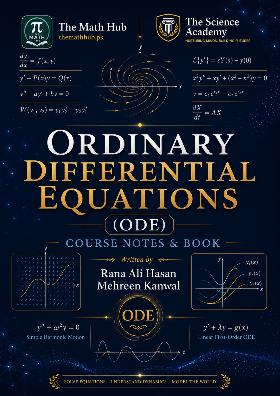
Ordinary Differential Equations (ODE) — Complete Course Notes & Book

A complete, easy-to-advanced course path from the language of differential equations and first-order methods to higher-order equations, Laplace transforms, series, special functions, systems, dynamical systems, boundary-value theory, numerical ODEs and asymptotic methods.

Course-name variants: Ordinary Differential Equation, ODE, ODEs, Differential Equations, Differential Equation, Elementary Differential Equations, ODE-I, ODE-II, Ordinary Differential Equations-I, Ordinary Differential Equations-II, Differential Equations and Dynamical Systems, Theory of Ordinary Differential Equations. These are legitimate discovery aliases; the canonical subject identity remains Ordinary Differential Equations (ODE), not separate ODE-I, ODE-II or Differential Equations doorway pages.

Prepared by Rana Ali Hasan — MPhil Mathematics and Mehreen Kanwal — MPhil Mathematics.

26 chapters239 A4 PDF pagesComplete course bookEnglishUpdated 01 September 2026
Ordinary Differential Equations (ODE) complete course notes and book by The Math Hub
Ordinary Differential Equations (ODE) · Course Notes & Book · The Math Hub
About this book

A complete Ordinary Differential Equations (ODE) learning path

The HTML resource is useful before the PDF is opened: it exposes the progression, chapter coverage, theorem and method vocabulary, curriculum context, references, FAQs and lawful resource actions.

What this resource covers

The book progresses from definitions, classification and first-order solution methods through existence and uniqueness, modelling, higher-order linear ODEs, constant coefficients, forced equations, mechanics, Laplace transforms, power series and Frobenius methods.

It then continues through special functions, systems, phase-plane analysis, nonlinear stability, global planar behaviour, Floquet theory, bifurcation, Green functions, Sturm–Liouville theory, numerical methods and perturbation/asymptotic methods.

Why study Ordinary Differential Equations?

ODEs describe change: motion, growth, decay, heat, circuits, populations, control systems and interacting components. The subject connects calculus and linear algebra with modelling, numerical analysis and dynamical systems.

Purpose and benefits

  • Build a reliable method-selection habit.
  • Keep theorem hypotheses, initial data and boundary conditions visible.
  • Move from symbolic solutions to qualitative and numerical interpretation.
  • Connect classroom ODE methods with scientific and engineering models.

Who this resource is for

ADP and associate-degree learners, BS Mathematics students, legacy BSc students, MSc revision learners, and physics, engineering, computing or data-science students who need ODE foundations.

Suggested readiness

Be comfortable with algebra, functions, differentiation, integration and basic matrices. The early chapters refresh the language; the later chapters can be selected according to the learner’s course and prerequisites.

Learning outcomes

Classify ODEs, IVPs and BVPs and verify proposed solutions.Select and apply separable, exact, linear, Bernoulli and special first-order methods.Solve higher-order constant- and variable-coefficient equations with appropriate checks.Use Laplace, power-series and Frobenius methods for structured IVPs and singular points.Analyse systems with eigenvalues, matrix exponentials, phase portraits and linearization.State and use existence, uniqueness, stability, spectral and numerical results with hypotheses.Interpret models in mechanics, circuits, biology, population dynamics and scientific computing.Compare numerical accuracy, stability, stiffness and asymptotic validity.
Course roadmap

Course Contents — 26 chapters

Each crawlable entry links to a separate detailed block below. Start with Chapters 1–7 for a first-course foundation, continue through Chapters 8–18 for higher-order, transform, series and systems work, and use Chapters 19–26 for advanced theory and computation.

  1. Chapter 01Introduction to Ordinary Differential Equations (ODE)
  2. Chapter 02Separable, Homogeneous and Reducible First-Order Equations
  3. Chapter 03Exact Equations, Integrating Factors and Linear ODEs
  4. Chapter 04Special Nonlinear First-Order Equations
  5. Chapter 05Geometrical and Qualitative Study of First-Order ODEs
  6. Chapter 06Existence, Uniqueness and Dependence of Solutions
  7. Chapter 07Mathematical Modelling with First-Order ODEs
  8. Chapter 08Theory of Higher-Order Linear Differential Equations
  9. Chapter 09Linear ODEs with Constant Coefficients
  10. Chapter 10Nonhomogeneous Linear ODEs
  11. Chapter 11Variable-Coefficient Higher-Order Equations
  12. Chapter 12Mechanical, Electrical and Physical Applications
  13. Chapter 13Laplace Transform Methods for ODEs
  14. Chapter 14Power-Series Solutions about Ordinary Points
  15. Chapter 15Singular Points and the Frobenius Method
  16. Chapter 16Special Differential Equations and Special Functions
  17. Chapter 17Systems of Linear Ordinary Differential Equations
  18. Chapter 18Phase-Plane Analysis of Linear Systems
  19. Chapter 19Nonlinear Autonomous Systems and Local Stability
  20. Chapter 20Global Behaviour of Planar Nonlinear Systems
  21. Chapter 21Periodic Linear Systems and Floquet Theory
  22. Chapter 22Bifurcation Theory and Advanced Dynamical Behaviour
  23. Chapter 23Boundary-Value Problems and Green’s Functions
  24. Chapter 24Sturm–Liouville Theory and Oscillation
  25. Chapter 25Numerical Solution of Ordinary Differential Equations
  26. Chapter 26Perturbation and Asymptotic Methods for ODEs
Chapter-by-chapter coverage

Detailed Ordinary Differential Equations (ODE) chapters

These 26 visible blocks represent the supplied academic structure with granular subtopics, purpose, learning outcomes, applications and chapter navigation. Chapter links open the complete book PDF because no separate chapter files are claimed.

Chapter 01

Chapter 01: Introduction to Ordinary Differential Equations (ODE)

Why this chapter is taught: Establish the language, classification, notation and problem types used throughout the course.

What is taught

  • Historical motivation and role of differential equations
  • Differential equations versus ordinary and partial differential equations
  • Dependent and independent variables
  • Order and degree
  • Linear and nonlinear ODEs
  • Autonomous and non-autonomous equations
  • Explicit and implicit forms
  • General, particular and singular solutions
  • Initial-value problems (IVPs)
  • Boundary-value problems (BVPs)
  • Verification of solutions
  • Formation of differential equations by elimination of arbitrary constants
  • Basic mathematical modelling
  • Notation y′, y″, dy/dx and operator notation

Learning outcomes and benefits

  • Explain the definitions, notation and central methods of Introduction to Ordinary Differential Equations (ODE).
  • Apply the chapter's principal techniques to representative problems and check the assumptions behind each method.
  • Move from guided worked examples to independent practice, interpreting the solution rather than only manipulating symbols.
  • Recognize when the chapter's method applies and when a different Ordinary Differential Equations (ODE) method is required.
  • Connect the chapter with earlier prerequisites and the later theory of the complete ODE course.

Applications and connections

  • Physics and engineering model formulation
  • Population and growth models
  • Later IVP and BVP theory

Read Chapter 01 in the complete ODE book PDF →

Chapter 02

Chapter 02: Separable, Homogeneous and Reducible First-Order Equations

Why this chapter is taught: Build the first practical solution toolkit and teach students to recognize separable and homogeneous structures.

What is taught

  • First-order normal form
  • Separation of variables
  • Implicit versus explicit solutions
  • Constant/equilibrium solutions in separable equations
  • Equations reducible to separable form
  • Homogeneous functions
  • First-order homogeneous equations dy/dx = F(y/x)
  • Substitutions y = vx and x = vy
  • Translation substitutions for reducible-to-homogeneous equations
  • Initial conditions and interval restrictions
  • Recognition strategy for selecting the method

Learning outcomes and benefits

  • Explain the definitions, notation and central methods of Separable, Homogeneous and Reducible First-Order Equations.
  • Apply the chapter's principal techniques to representative problems and check the assumptions behind each method.
  • Move from guided worked examples to independent practice, interpreting the solution rather than only manipulating symbols.
  • Recognize when the chapter's method applies and when a different Ordinary Differential Equations (ODE) method is required.
  • Connect the chapter with earlier prerequisites and the later theory of the complete ODE course.

Applications and connections

  • Growth and decay
  • Elementary mechanics
  • Mixing and rate models

Read Chapter 02 in the complete ODE book PDF →

Chapter 03

Chapter 03: Exact Equations, Integrating Factors and Linear ODEs

Why this chapter is taught: Develop systematic exactness, integrating-factor and first-order linear techniques.

What is taught

  • Differential form M dx + N dy = 0
  • Exact differential equations
  • Exactness criterion M_y = N_x
  • Potential-function construction
  • Integration strategy for exact equations
  • Integrating factors
  • Integrating factors depending on x or y
  • First-order linear equations y′ + P(x)y = Q(x)
  • Integrating factor exp(∫P dx)
  • Initial-value problems for linear equations
  • Bernoulli equation and reduction to linear form
  • Method recognition and verification

Learning outcomes and benefits

  • Explain the definitions, notation and central methods of Exact Equations, Integrating Factors and Linear ODEs.
  • Apply the chapter's principal techniques to representative problems and check the assumptions behind each method.
  • Move from guided worked examples to independent practice, interpreting the solution rather than only manipulating symbols.
  • Recognize when the chapter's method applies and when a different Ordinary Differential Equations (ODE) method is required.
  • Connect the chapter with earlier prerequisites and the later theory of the complete ODE course.

Applications and connections

  • Circuits and input-response models
  • Cooling and mixing
  • Linear rate processes

Read Chapter 03 in the complete ODE book PDF →

Chapter 04

Chapter 04: Special Nonlinear First-Order Equations

Why this chapter is taught: Extend first-order solving beyond first-degree and linear patterns and introduce singular-solution geometry.

What is taught

  • First-order equations not necessarily first degree
  • Equations solvable for p = dy/dx
  • Equations solvable for x
  • Equations solvable for y
  • Clairaut equation
  • Singular solutions and envelopes
  • Lagrange or d’Alembert-type equations
  • Riccati equation
  • Riccati reduction when a particular solution is known
  • Abel-type first-order equations as advanced enrichment
  • Singular-solution tests
  • Geometric interpretation where useful

Learning outcomes and benefits

  • Explain the definitions, notation and central methods of Special Nonlinear First-Order Equations.
  • Apply the chapter's principal techniques to representative problems and check the assumptions behind each method.
  • Move from guided worked examples to independent practice, interpreting the solution rather than only manipulating symbols.
  • Recognize when the chapter's method applies and when a different Ordinary Differential Equations (ODE) method is required.
  • Connect the chapter with earlier prerequisites and the later theory of the complete ODE course.

Applications and connections

  • Envelopes and singular solutions
  • Riccati transformations
  • Special nonlinear models

Read Chapter 04 in the complete ODE book PDF →

Chapter 05

Chapter 05: Geometrical and Qualitative Study of First-Order ODEs

Why this chapter is taught: Teach students to understand solution behavior graphically and qualitatively even when closed-form solutions are unavailable.

What is taught

  • Direction fields and slope fields
  • Isoclines
  • Integral curves
  • Autonomous scalar equations
  • Equilibrium solutions
  • Phase-line analysis
  • Stable, unstable and semistable equilibria
  • Long-term behavior without explicit solution
  • Nullclines in scalar context
  • Qualitative comparison of solution families
  • Elementary scalar bifurcations
  • Graphical versus analytic solution viewpoints

Learning outcomes and benefits

  • Explain the definitions, notation and central methods of Geometrical and Qualitative Study of First-Order ODEs.
  • Apply the chapter's principal techniques to representative problems and check the assumptions behind each method.
  • Move from guided worked examples to independent practice, interpreting the solution rather than only manipulating symbols.
  • Recognize when the chapter's method applies and when a different Ordinary Differential Equations (ODE) method is required.
  • Connect the chapter with earlier prerequisites and the later theory of the complete ODE course.

Applications and connections

  • Qualitative prediction
  • Stability screening
  • Preparation for bifurcation analysis

Read Chapter 05 in the complete ODE book PDF →

Chapter 06

Chapter 06: Existence, Uniqueness and Dependence of Solutions

Why this chapter is taught: Provide the theoretical foundation for when IVPs have solutions, when those solutions are unique, and how they depend on data.

What is taught

  • Domains and initial-value problems
  • Continuity conditions
  • Lipschitz condition
  • Local existence
  • Peano existence theorem
  • Picard successive approximations
  • Picard–Lindelöf existence and uniqueness theorem
  • Banach fixed-point viewpoint where appropriate
  • Grönwall inequality
  • Uniqueness consequences
  • Maximal interval of existence
  • Continuation and extensibility
  • Finite-time blow-up
  • Continuous dependence on initial data
  • Continuous dependence on parameters
  • Comparison principles
  • Differential inequalities

Learning outcomes and benefits

  • Explain the definitions, notation and central methods of Existence, Uniqueness and Dependence of Solutions.
  • Apply the chapter's principal techniques to representative problems and check the assumptions behind each method.
  • Move from guided worked examples to independent practice, interpreting the solution rather than only manipulating symbols.
  • Recognize when the chapter's method applies and when a different Ordinary Differential Equations (ODE) method is required.
  • Connect the chapter with earlier prerequisites and the later theory of the complete ODE course.

Applications and connections

  • Well-posedness of models
  • Justification of numerical methods
  • Stability and perturbation analysis

Read Chapter 06 in the complete ODE book PDF →

Chapter 07

Chapter 07: Mathematical Modelling with First-Order ODEs

Why this chapter is taught: Turn first-order ODE techniques into mathematical models for real changing systems.

What is taught

  • Model-building workflow and units
  • Exponential growth and decay
  • Radioactive decay and carbon dating
  • Population growth
  • Logistic equation
  • Harvesting models
  • Newton law of cooling and heating
  • Mixing problems
  • Falling bodies and resistance
  • Chemical/reaction models
  • Compound interest and simple economic models
  • Basic biological models
  • Orthogonal trajectories
  • Isogonal trajectories where useful
  • Interpretation and validation of models

Learning outcomes and benefits

  • Explain the definitions, notation and central methods of Mathematical Modelling with First-Order ODEs.
  • Apply the chapter's principal techniques to representative problems and check the assumptions behind each method.
  • Move from guided worked examples to independent practice, interpreting the solution rather than only manipulating symbols.
  • Recognize when the chapter's method applies and when a different Ordinary Differential Equations (ODE) method is required.
  • Connect the chapter with earlier prerequisites and the later theory of the complete ODE course.

Applications and connections

  • Population dynamics
  • Radioactive decay
  • Heat transfer
  • Mixing tanks
  • Economics and biology

Read Chapter 07 in the complete ODE book PDF →

Chapter 08

Chapter 08: Theory of Higher-Order Linear Differential Equations

Why this chapter is taught: Build the general vector-space theory behind higher-order linear ODEs.

What is taught

  • nth-order ODEs
  • Linear differential operators
  • Homogeneous and nonhomogeneous equations
  • Higher-order IVPs and BVPs
  • Superposition principle
  • Linear independence and dependence of solutions
  • Fundamental solution sets
  • Wronskian
  • Abel identity
  • Existence and uniqueness for linear nth-order IVPs
  • Dimension of the solution space
  • Fundamental theorem structure and hypotheses

Learning outcomes and benefits

  • Explain the definitions, notation and central methods of Theory of Higher-Order Linear Differential Equations.
  • Apply the chapter's principal techniques to representative problems and check the assumptions behind each method.
  • Move from guided worked examples to independent practice, interpreting the solution rather than only manipulating symbols.
  • Recognize when the chapter's method applies and when a different Ordinary Differential Equations (ODE) method is required.
  • Connect the chapter with earlier prerequisites and the later theory of the complete ODE course.

Applications and connections

  • Mechanics and circuits
  • Reduction of systems to scalar equations
  • Boundary-value theory

Read Chapter 08 in the complete ODE book PDF →

Chapter 09

Chapter 09: Linear ODEs with Constant Coefficients

Why this chapter is taught: Master the characteristic-equation approach for constant-coefficient linear equations.

What is taught

  • Characteristic or auxiliary equation
  • Distinct real roots
  • Repeated real roots
  • Complex-conjugate roots
  • Repeated complex roots
  • Differential-operator D notation
  • Complementary function
  • Particular integral viewpoint
  • Operator shortcuts
  • Initial conditions
  • Resonance cases
  • Higher-order constant-coefficient equations

Learning outcomes and benefits

  • Explain the definitions, notation and central methods of Linear ODEs with Constant Coefficients.
  • Apply the chapter's principal techniques to representative problems and check the assumptions behind each method.
  • Move from guided worked examples to independent practice, interpreting the solution rather than only manipulating symbols.
  • Recognize when the chapter's method applies and when a different Ordinary Differential Equations (ODE) method is required.
  • Connect the chapter with earlier prerequisites and the later theory of the complete ODE course.

Applications and connections

  • Vibration models
  • RLC circuits
  • Control-system transients

Read Chapter 09 in the complete ODE book PDF →

Chapter 10

Chapter 10: Nonhomogeneous Linear ODEs

Why this chapter is taught: Solve forced linear equations and compare the major particular-solution techniques.

What is taught

  • Superposition for forcing terms
  • Method of undetermined coefficients
  • Polynomial forcing
  • Exponential forcing
  • Trigonometric forcing
  • Products of standard forcing types
  • Resonance adjustments
  • Annihilator method
  • Variation of parameters for second-order equations
  • Variation of parameters for higher-order equations
  • Method comparison and selection
  • Verification of particular solutions

Learning outcomes and benefits

  • Explain the definitions, notation and central methods of Nonhomogeneous Linear ODEs.
  • Apply the chapter's principal techniques to representative problems and check the assumptions behind each method.
  • Move from guided worked examples to independent practice, interpreting the solution rather than only manipulating symbols.
  • Recognize when the chapter's method applies and when a different Ordinary Differential Equations (ODE) method is required.
  • Connect the chapter with earlier prerequisites and the later theory of the complete ODE course.

Applications and connections

  • Forced oscillations
  • External inputs
  • Engineering response models

Read Chapter 10 in the complete ODE book PDF →

Chapter 11

Chapter 11: Variable-Coefficient Higher-Order Equations

Why this chapter is taught: Handle important variable-coefficient higher-order equations and structural transformations.

What is taught

  • Reduction of order
  • Construction of a second solution from a known solution
  • Cauchy–Euler or equidimensional equations
  • Transformations for Euler equations
  • Change of dependent variable
  • Change of independent variable
  • Reduction to normal form
  • Self-adjoint form
  • Riccati connection to second-order linear equations
  • Variable-coefficient method selection

Learning outcomes and benefits

  • Explain the definitions, notation and central methods of Variable-Coefficient Higher-Order Equations.
  • Apply the chapter's principal techniques to representative problems and check the assumptions behind each method.
  • Move from guided worked examples to independent practice, interpreting the solution rather than only manipulating symbols.
  • Recognize when the chapter's method applies and when a different Ordinary Differential Equations (ODE) method is required.
  • Connect the chapter with earlier prerequisites and the later theory of the complete ODE course.

Applications and connections

  • Scale-invariant models
  • Special-function reductions
  • Mathematical physics

Read Chapter 11 in the complete ODE book PDF →

Chapter 12

Chapter 12: Mechanical, Electrical and Physical Applications

Why this chapter is taught: Connect second-order ODEs to oscillations, circuits and measurable physical parameters.

What is taught

  • Simple harmonic motion
  • Free undamped motion
  • Damped motion
  • Overdamping
  • Critical damping
  • Underdamping
  • Forced oscillations
  • Resonance
  • Beats
  • Spring-mass systems
  • RLC circuits
  • Mechanical-electrical analogies
  • Coupled oscillations introduction
  • Transient and steady-state behavior
  • Parameter interpretation

Learning outcomes and benefits

  • Explain the definitions, notation and central methods of Mechanical, Electrical and Physical Applications.
  • Apply the chapter's principal techniques to representative problems and check the assumptions behind each method.
  • Move from guided worked examples to independent practice, interpreting the solution rather than only manipulating symbols.
  • Recognize when the chapter's method applies and when a different Ordinary Differential Equations (ODE) method is required.
  • Connect the chapter with earlier prerequisites and the later theory of the complete ODE course.

Applications and connections

  • Mechanical vibration
  • Electrical circuits
  • Resonance and damping

Read Chapter 12 in the complete ODE book PDF →

Chapter 13

Chapter 13: Laplace Transform Methods for ODEs

Why this chapter is taught: Solve IVPs with discontinuous, impulsive and piecewise forcing using transform methods.

What is taught

  • Definition of Laplace transform
  • Conditions for existence
  • Basic transform table
  • Linearity
  • First shifting theorem
  • Second shifting theorem
  • Transform of derivatives
  • Transform of integrals
  • Inverse Laplace transforms
  • Partial fractions
  • Solution of IVPs
  • Heaviside unit-step functions
  • Piecewise forcing
  • Dirac delta and impulse
  • Convolution theorem
  • Impulse response
  • Transfer functions and poles
  • Periodic forcing

Learning outcomes and benefits

  • Explain the definitions, notation and central methods of Laplace Transform Methods for ODEs.
  • Apply the chapter's principal techniques to representative problems and check the assumptions behind each method.
  • Move from guided worked examples to independent practice, interpreting the solution rather than only manipulating symbols.
  • Recognize when the chapter's method applies and when a different Ordinary Differential Equations (ODE) method is required.
  • Connect the chapter with earlier prerequisites and the later theory of the complete ODE course.

Applications and connections

  • Switching circuits
  • Impulse response
  • Control and transfer functions

Read Chapter 13 in the complete ODE book PDF →

Chapter 14

Chapter 14: Power-Series Solutions about Ordinary Points

Why this chapter is taught: Develop series solutions around ordinary points when elementary closed forms are unavailable.

What is taught

  • Review of power series
  • Radius and interval of convergence
  • Term-by-term differentiation and integration
  • Analytic coefficients
  • Ordinary points
  • Assumed-series solutions
  • Index shifting
  • Coefficient matching
  • Recurrence relations
  • Two linearly independent series solutions
  • Initial conditions with series methods
  • Analytic-solution existence near ordinary points

Learning outcomes and benefits

  • Explain the definitions, notation and central methods of Power-Series Solutions about Ordinary Points.
  • Apply the chapter's principal techniques to representative problems and check the assumptions behind each method.
  • Move from guided worked examples to independent practice, interpreting the solution rather than only manipulating symbols.
  • Recognize when the chapter's method applies and when a different Ordinary Differential Equations (ODE) method is required.
  • Connect the chapter with earlier prerequisites and the later theory of the complete ODE course.

Applications and connections

  • Local analytic approximations
  • Special functions
  • Numerical benchmarking

Read Chapter 14 in the complete ODE book PDF →

Chapter 15

Chapter 15: Singular Points and the Frobenius Method

Why this chapter is taught: Extend series methods to regular singular points through Frobenius theory.

What is taught

  • Singular points
  • Regular singular points
  • Irregular singular points
  • Frobenius form
  • Indicial equation
  • Distinct indicial roots not differing by an integer
  • Roots differing by an integer
  • Repeated indicial roots
  • Logarithmic second solutions
  • Frobenius theorem
  • Convergence issues
  • Fuchs-type perspective as enrichment

Learning outcomes and benefits

  • Explain the definitions, notation and central methods of Singular Points and the Frobenius Method.
  • Apply the chapter's principal techniques to representative problems and check the assumptions behind each method.
  • Move from guided worked examples to independent practice, interpreting the solution rather than only manipulating symbols.
  • Recognize when the chapter's method applies and when a different Ordinary Differential Equations (ODE) method is required.
  • Connect the chapter with earlier prerequisites and the later theory of the complete ODE course.

Applications and connections

  • Bessel- and Legendre-type equations
  • Singular-point analysis
  • Mathematical physics

Read Chapter 15 in the complete ODE book PDF →

Chapter 16

Chapter 16: Special Differential Equations and Special Functions

Why this chapter is taught: Connect ODEs with classical special functions used throughout mathematical physics.

What is taught

  • Bessel equation
  • Bessel functions Jν
  • Second independent Bessel solutions Yν
  • Bessel recurrence relations and identities
  • Modified Bessel equation
  • Modified Bessel functions Iν and Kν
  • Legendre equation
  • Legendre polynomials
  • Associated Legendre equation
  • Hermite equation and Hermite polynomials
  • Laguerre equation and Laguerre polynomials
  • Airy equation and Airy functions
  • Chebyshev differential equation
  • Hypergeometric equation
  • Confluent hypergeometric connection
  • Generating functions
  • Orthogonality properties
  • Applications of special functions

Learning outcomes and benefits

  • Explain the definitions, notation and central methods of Special Differential Equations and Special Functions.
  • Apply the chapter's principal techniques to representative problems and check the assumptions behind each method.
  • Move from guided worked examples to independent practice, interpreting the solution rather than only manipulating symbols.
  • Recognize when the chapter's method applies and when a different Ordinary Differential Equations (ODE) method is required.
  • Connect the chapter with earlier prerequisites and the later theory of the complete ODE course.

Applications and connections

  • Cylindrical and spherical models
  • Quantum and wave problems
  • Orthogonal expansions

Read Chapter 16 in the complete ODE book PDF →

Chapter 17

Chapter 17: Systems of Linear Ordinary Differential Equations

Why this chapter is taught: Move from scalar equations to vector systems and matrix-based solution theory.

What is taught

  • Systems as vector ODEs
  • Conversion of higher-order ODEs to first-order systems
  • Existence and uniqueness for systems
  • Linear homogeneous systems
  • Fundamental solution matrix
  • Fundamental matrix properties
  • Determinant and Wronskian of a system
  • Liouville formula
  • Constant-coefficient matrix systems
  • Eigenvalue-eigenvector method
  • Distinct real eigenvalues
  • Complex eigenvalues
  • Repeated eigenvalues
  • Generalized eigenvectors and Jordan chains
  • Matrix exponential exp(At)
  • Nonhomogeneous systems
  • Variation-of-constants formula
  • Elimination and operator methods

Learning outcomes and benefits

  • Explain the definitions, notation and central methods of Systems of Linear Ordinary Differential Equations.
  • Apply the chapter's principal techniques to representative problems and check the assumptions behind each method.
  • Move from guided worked examples to independent practice, interpreting the solution rather than only manipulating symbols.
  • Recognize when the chapter's method applies and when a different Ordinary Differential Equations (ODE) method is required.
  • Connect the chapter with earlier prerequisites and the later theory of the complete ODE course.

Applications and connections

  • Coupled systems
  • State-space models
  • Control, networks and multicomponent dynamics

Read Chapter 17 in the complete ODE book PDF →

Chapter 18

Chapter 18: Phase-Plane Analysis of Linear Systems

Why this chapter is taught: Classify the geometry and stability of two-dimensional linear systems.

What is taught

  • Phase space, trajectories and orbits
  • Equilibrium points
  • Eigenvector directions
  • Stable nodes
  • Unstable nodes
  • Saddles
  • Spirals and foci
  • Centers
  • Degenerate repeated-eigenvalue cases
  • Defective systems
  • Trace-determinant plane
  • Phase portraits
  • Stable and unstable subspaces
  • Classification from eigenvalues

Learning outcomes and benefits

  • Explain the definitions, notation and central methods of Phase-Plane Analysis of Linear Systems.
  • Apply the chapter's principal techniques to representative problems and check the assumptions behind each method.
  • Move from guided worked examples to independent practice, interpreting the solution rather than only manipulating symbols.
  • Recognize when the chapter's method applies and when a different Ordinary Differential Equations (ODE) method is required.
  • Connect the chapter with earlier prerequisites and the later theory of the complete ODE course.

Applications and connections

  • Stability of linear models
  • Phase portraits
  • Local approximations to nonlinear systems

Read Chapter 18 in the complete ODE book PDF →

Chapter 19

Chapter 19: Nonlinear Autonomous Systems and Local Stability

Why this chapter is taught: Develop local nonlinear stability theory using linearization and Lyapunov methods.

What is taught

  • Autonomous systems
  • Flows
  • Equilibria and fixed points
  • Jacobian matrix
  • Linearization
  • Hyperbolic equilibria
  • Hartman–Grobman theorem
  • Stability definitions
  • Lyapunov stability
  • Asymptotic stability
  • Exponential stability
  • Lyapunov indirect method
  • Lyapunov direct method
  • Lyapunov functions
  • LaSalle invariance principle
  • Stable and unstable manifolds introduction

Learning outcomes and benefits

  • Explain the definitions, notation and central methods of Nonlinear Autonomous Systems and Local Stability.
  • Apply the chapter's principal techniques to representative problems and check the assumptions behind each method.
  • Move from guided worked examples to independent practice, interpreting the solution rather than only manipulating symbols.
  • Recognize when the chapter's method applies and when a different Ordinary Differential Equations (ODE) method is required.
  • Connect the chapter with earlier prerequisites and the later theory of the complete ODE course.

Applications and connections

  • Nonlinear control and stability
  • Ecology and mechanics
  • Local dynamical systems

Read Chapter 19 in the complete ODE book PDF →

Chapter 20

Chapter 20: Global Behaviour of Planar Nonlinear Systems

Why this chapter is taught: Study global planar dynamics, limit sets, periodic orbits and invariant geometry.

What is taught

  • Nullclines
  • Direction fields for systems
  • Invariant regions
  • Positive invariance
  • Orbits and limit sets
  • Alpha- and omega-limit sets
  • Periodic orbits
  • Limit cycles
  • Poincaré–Bendixson theorem
  • Bendixson criterion
  • Bendixson–Dulac criterion
  • Hamiltonian systems
  • Conservative systems
  • Gradient systems
  • Lotka–Volterra model
  • Predator-prey phase plane
  • Competition models

Learning outcomes and benefits

  • Explain the definitions, notation and central methods of Global Behaviour of Planar Nonlinear Systems.
  • Apply the chapter's principal techniques to representative problems and check the assumptions behind each method.
  • Move from guided worked examples to independent practice, interpreting the solution rather than only manipulating symbols.
  • Recognize when the chapter's method applies and when a different Ordinary Differential Equations (ODE) method is required.
  • Connect the chapter with earlier prerequisites and the later theory of the complete ODE course.

Applications and connections

  • Population competition
  • Predator-prey dynamics
  • Limit cycles and conservative systems

Read Chapter 20 in the complete ODE book PDF →

Chapter 21

Chapter 21: Periodic Linear Systems and Floquet Theory

Why this chapter is taught: Analyze linear systems with periodic coefficients and parametric resonance.

What is taught

  • Linear ODEs with periodic coefficients
  • Fundamental matrices for periodic systems
  • Monodromy matrix
  • Floquet multipliers
  • Floquet exponents
  • Floquet theorem
  • Stability via Floquet multipliers
  • Periodic nonhomogeneous solutions
  • Poincaré maps
  • Mathieu equation
  • Hill equation
  • Parametric resonance

Learning outcomes and benefits

  • Explain the definitions, notation and central methods of Periodic Linear Systems and Floquet Theory.
  • Apply the chapter's principal techniques to representative problems and check the assumptions behind each method.
  • Move from guided worked examples to independent practice, interpreting the solution rather than only manipulating symbols.
  • Recognize when the chapter's method applies and when a different Ordinary Differential Equations (ODE) method is required.
  • Connect the chapter with earlier prerequisites and the later theory of the complete ODE course.

Applications and connections

  • Periodic forcing
  • Parametric resonance
  • Vibrations and stability

Read Chapter 21 in the complete ODE book PDF →

Chapter 22

Chapter 22: Bifurcation Theory and Advanced Dynamical Behaviour

Why this chapter is taught: Understand how qualitative dynamics change as parameters vary, including local bifurcations.

What is taught

  • Parameters and qualitative change
  • Saddle-node bifurcation
  • Transcritical bifurcation
  • Pitchfork bifurcation
  • Hopf bifurcation
  • Normal forms
  • Center-manifold idea
  • Stable and unstable manifolds
  • Homoclinic trajectories
  • Heteroclinic trajectories
  • Poincaré return maps
  • Period-doubling idea
  • Deterministic chaos introduction
  • Sensitive dependence
  • Lorenz-type example as enrichment

Learning outcomes and benefits

  • Explain the definitions, notation and central methods of Bifurcation Theory and Advanced Dynamical Behaviour.
  • Apply the chapter's principal techniques to representative problems and check the assumptions behind each method.
  • Move from guided worked examples to independent practice, interpreting the solution rather than only manipulating symbols.
  • Recognize when the chapter's method applies and when a different Ordinary Differential Equations (ODE) method is required.
  • Connect the chapter with earlier prerequisites and the later theory of the complete ODE course.

Applications and connections

  • Threshold phenomena
  • Onset of oscillation
  • Qualitative parameter sensitivity

Read Chapter 22 in the complete ODE book PDF →

Chapter 23

Chapter 23: Boundary-Value Problems and Green’s Functions

Why this chapter is taught: Develop two-point boundary-value theory and the Green-function solution framework.

What is taught

  • Initial versus boundary conditions
  • Two-point boundary-value problems
  • Dirichlet conditions
  • Neumann conditions
  • Robin or mixed conditions
  • Homogeneous BVPs
  • Nonhomogeneous BVPs
  • Existence, nonexistence and nonuniqueness
  • Resonance and compatibility
  • Eigenvalue-type BVPs
  • Green’s function concept
  • Construction of Green’s functions
  • Continuity and derivative jump conditions
  • Solution representation with Green’s function
  • Symmetry in self-adjoint cases
  • Shooting method
  • Integral formulation
  • Fredholm-alternative perspective

Learning outcomes and benefits

  • Explain the definitions, notation and central methods of Boundary-Value Problems and Green’s Functions.
  • Apply the chapter's principal techniques to representative problems and check the assumptions behind each method.
  • Move from guided worked examples to independent practice, interpreting the solution rather than only manipulating symbols.
  • Recognize when the chapter's method applies and when a different Ordinary Differential Equations (ODE) method is required.
  • Connect the chapter with earlier prerequisites and the later theory of the complete ODE course.

Applications and connections

  • Heat and vibration eigenproblems after separation
  • Forced BVPs
  • Operator and integral methods

Read Chapter 23 in the complete ODE book PDF →

Chapter 24

Chapter 24: Sturm–Liouville Theory and Oscillation

Why this chapter is taught: Build the spectral theory of self-adjoint second-order problems and their oscillation properties.

What is taught

  • Sturm–Liouville differential operator
  • Adjoint operators
  • Self-adjoint operators
  • Lagrange identity and boundary form
  • Regular Sturm–Liouville problems
  • Separated boundary conditions
  • Eigenvalues and eigenfunctions
  • Reality of eigenvalues
  • Simplicity properties
  • Orthogonality of eigenfunctions
  • Weight functions
  • Rayleigh quotient
  • Eigenfunction expansions
  • Sturm separation theorem
  • Sturm comparison theorem
  • Oscillation and nodal theorems
  • Ordering of eigenvalues
  • Completeness perspective
  • Singular Sturm–Liouville problems
  • Spectral Green functions
  • Connections with Fourier expansions

Learning outcomes and benefits

  • Explain the definitions, notation and central methods of Sturm–Liouville Theory and Oscillation.
  • Apply the chapter's principal techniques to representative problems and check the assumptions behind each method.
  • Move from guided worked examples to independent practice, interpreting the solution rather than only manipulating symbols.
  • Recognize when the chapter's method applies and when a different Ordinary Differential Equations (ODE) method is required.
  • Connect the chapter with earlier prerequisites and the later theory of the complete ODE course.

Applications and connections

  • Fourier-type expansions
  • Quantum and mechanical eigenproblems
  • PDE separation of variables

Read Chapter 24 in the complete ODE book PDF →

Chapter 25

Chapter 25: Numerical Solution of Ordinary Differential Equations

Why this chapter is taught: Compute reliable approximate ODE solutions and understand consistency, stability, convergence and stiffness.

What is taught

  • Why numerical methods are needed
  • Well-posed IVPs
  • Local and global truncation error
  • Euler method
  • Modified Euler method
  • Improved Euler or Heun method
  • Midpoint method
  • Taylor-series methods
  • Runge–Kutta methods
  • Classical RK4
  • Embedded and adaptive Runge–Kutta concepts
  • Multistep methods
  • Adams–Bashforth methods
  • Adams–Moulton methods
  • Predictor–corrector methods
  • Milne–Simpson method
  • Consistency
  • Convergence
  • Zero-stability
  • Dahlquist equivalence theorem
  • Absolute stability
  • A-stability
  • L-stability
  • Stiff differential equations
  • Backward differentiation formulas
  • Numerical solution of systems
  • Shooting method for BVPs
  • Finite-difference treatment of BVPs
  • Error comparison and computational experiments

Learning outcomes and benefits

  • Explain the definitions, notation and central methods of Numerical Solution of Ordinary Differential Equations.
  • Apply the chapter's principal techniques to representative problems and check the assumptions behind each method.
  • Move from guided worked examples to independent practice, interpreting the solution rather than only manipulating symbols.
  • Recognize when the chapter's method applies and when a different Ordinary Differential Equations (ODE) method is required.
  • Connect the chapter with earlier prerequisites and the later theory of the complete ODE course.

Applications and connections

  • Engineering simulation
  • Scientific computing
  • Stiff models
  • Numerical BVPs

Read Chapter 25 in the complete ODE book PDF →

Chapter 26

Chapter 26: Perturbation and Asymptotic Methods for ODEs

Why this chapter is taught: Introduce systematic approximations for ODEs containing small parameters or multiple scales.

What is taught

  • Small parameters in ODEs
  • Regular perturbation
  • Breakdown and secular terms
  • Poincaré–Lindstedt method
  • Method of multiple scales
  • Averaging method
  • Singular perturbations
  • Boundary-layer ideas
  • Matched asymptotic expansions
  • Composite expansions
  • WKB approximation
  • Turning points and Airy scaling
  • Slowly varying oscillations
  • Resonance in perturbation problems
  • Asymptotic validity and error interpretation

Learning outcomes and benefits

  • Explain the definitions, notation and central methods of Perturbation and Asymptotic Methods for ODEs.
  • Apply the chapter's principal techniques to representative problems and check the assumptions behind each method.
  • Move from guided worked examples to independent practice, interpreting the solution rather than only manipulating symbols.
  • Recognize when the chapter's method applies and when a different Ordinary Differential Equations (ODE) method is required.
  • Connect the chapter with earlier prerequisites and the later theory of the complete ODE course.

Applications and connections

  • Weakly nonlinear oscillations
  • Boundary layers
  • High-frequency asymptotics
  • Singularly perturbed systems

Read Chapter 26 in the complete ODE book PDF →

Proof, theory and problem-solving scope

Important theorems, results and methods

Only named results and techniques represented in the supplied 26-chapter ODE scope are listed here. The final PDF remains the authority for the exact statement, proof depth and exercise treatment.

Important theorems and results

  • Peano Existence Theorem
  • Picard–Lindelöf Existence and Uniqueness Theorem
  • Picard successive-approximation construction
  • Grönwall Inequality
  • Comparison principles for scalar ODEs
  • Continuation and maximal-existence result
  • Continuous dependence on initial data and parameters
  • Superposition Principle
  • Existence and uniqueness theorem for linear nth-order IVPs
  • Wronskian criterion with hypotheses
  • Abel’s Identity
  • Variation-of-constants formula
  • Liouville Formula for systems
  • Frobenius Theorem
  • Hartman–Grobman Theorem
  • Lyapunov stability definitions and direct/indirect methods
  • LaSalle Invariance Principle
  • Poincaré–Bendixson Theorem
  • Bendixson and Bendixson–Dulac criteria
  • Floquet Theorem
  • Sturm–Liouville real-eigenvalue and orthogonality results
  • Rayleigh quotient perspective
  • Sturm Separation and Comparison Theorems
  • Oscillation and nodal results
  • Green-function continuity and derivative-jump construction
  • Dahlquist equivalence theorem: consistency plus zero-stability implies convergence where treated

Important solution methods and techniques

  • Separation of variables
  • Homogeneous substitution
  • Exact-equation potential method
  • Integrating-factor method
  • First-order linear method
  • Bernoulli substitution
  • Clairaut, Lagrange and Riccati special methods
  • Direction fields and phase lines
  • Picard iteration
  • Characteristic-equation method
  • Undetermined coefficients
  • Annihilator method
  • Variation of parameters
  • Reduction of order
  • Cauchy–Euler method
  • Laplace transforms
  • Unit-step and impulse forcing
  • Convolution
  • Power-series method
  • Frobenius method
  • Special-function recurrence methods
  • Matrix eigenvalue method
  • Matrix exponential
  • Variation of constants for systems
  • Phase-plane classification
  • Linearization
  • Lyapunov direct and indirect methods
  • Nullclines and invariant regions
  • Floquet multipliers
  • Normal forms and bifurcation analysis
  • Green functions
  • Shooting method
  • Sturm–Liouville eigenfunction expansion
  • Euler, Heun and midpoint methods
  • Runge–Kutta methods
  • Adams–Bashforth and Adams–Moulton methods
  • Predictor–corrector methods
  • BDF methods
  • Finite-difference BVP methods
  • Regular perturbation
  • Poincaré–Lindstedt method
  • Multiple scales
  • Averaging
  • Matched asymptotic expansions
  • WKB approximation

Worked examples and exercises

The course is organised for worked-example learning: classify the equation or system, choose a justified method, carry the initial or boundary data through the calculation, verify the result where possible, and interpret the outcome. Practice moves from elementary first-order calculations to theorem-based arguments, phase portraits, numerical error/stability comparisons and asymptotic approximations.

Applications and connections

Where Ordinary Differential Equations connect

Modelling

Growth, decay, logistic populations, harvesting, cooling, mixing, chemical reactions, falling bodies and basic economic or biological models translate assumptions into equations.

Mechanics and circuits

Second-order ODEs describe spring-mass motion, damping, resonance, beats, forced oscillations and RLC circuits, including transient and steady-state behaviour.

Analysis and physics

Power series, Frobenius, Bessel, Legendre, Hermite and other special equations support cylindrical, spherical, wave, quantum and eigenvalue problems.

Computing and systems

Matrix exponentials, phase planes, stability, numerical solvers, stiffness, BVP shooting and finite differences support control, simulation and scientific computing.

How to use this book

  1. Begin with definitions, notation and the classification checklist.
  2. Work Chapters 2–7 for first-order methods, qualitative ideas and modelling.
  3. Continue through Chapters 8–13 for higher-order equations, applications and Laplace methods.
  4. Use Chapters 14–18 for series, special functions and linear systems.
  5. Select Chapters 19–26 for dynamical systems, BVPs, Sturm–Liouville, numerical and asymptotic study.
  6. Use the HTML page for navigation and the PDF for the complete mathematical treatment.
Discovery and curriculum context

Programme relevance and placement

Every card below points to this same canonical HTML page. It is a discovery placement for relevant programmes, not a cloned course page, official university book or endorsement.

Pakistan course discovery evidence

Pakistan University / Course Crosswalk

University names, course codes and topic descriptions are curriculum/discovery context only. They do not imply endorsement, affiliation, official status or that this is an institution’s official book; confirm current schemes from each university.

Higher Education Commission (HEC) Pakistan

Course context: Mathematics Curriculum 2025 — national curriculum benchmark

ODE-related learning outcomes include modern analytical, series, Sturm–Liouville, modelling and qualitative/dynamical themes.

Official/source evidence →

University of Sargodha

Course context: MATH-6114 Ordinary Differential Equations

First-order methods, existence/uniqueness, higher-order equations, systems, power/Frobenius series, Bessel, modified Bessel, Legendre, Hermite and regular/singular Sturm–Liouville problems.

Official/source evidence →

University of the Punjab

Course context: Ordinary Differential Equations in Mathematics course structures

Preserved course material includes first/second-order ODEs, Sturm–Liouville systems, series and special differential equations.

Official/source evidence →

Quaid-i-Azam University

Course context: MA-305 Ordinary Differential Equations

BS Mathematics places Differential Equations and Linear Algebra earlier in the pathway and PDE later.

Official/source evidence →

COMSATS University Islamabad

Course context: MTH241 Ordinary Differential Equations

ODE appears in programme schemes and is used as a prerequisite for later PDE in Mathematics pathways.

Official/source evidence →

University of Central Punjab

Course context: Ordinary Differential Equations course outline

Coverage includes classification, existence/uniqueness, IVPs/BVPs, first-order methods, modelling, systems and power-series methods.

Official/source evidence →

The University of Lahore

Course context: Ordinary Differential Equations-I and Ordinary Differential Equations-II

The BS Mathematics pathway uses the ODE-I/ODE-II naming in its Sargodha-campus roadmap and current Mathematics programme context.

Official/source evidence →

University of Management and Technology (UMT)

Course context: MA-218 Ordinary Differential Equations; graduate Analysis of ODE

The BS Mathematics curriculum includes Ordinary Differential Equations and graduate listings include Analysis of Ordinary Differential Equations.

Official/source evidence →

University of Karachi

Course context: Ordinary Differential Equation course and syllabus material

Course material covers higher-order linear ODEs, systems, Green functions, power series and numerical ODE methods.

Official/source evidence →

International Islamic University Islamabad (IIUI)

Course context: MATH-342 Ordinary Differential Equations

Programme evidence lists ODE; engineering mathematics also uses linear ordinary differential equations and related modelling.

Official/source evidence →

University of Gujrat

Course context: Elementary Differential Equations and MATH-307 Ordinary Differential Equations

The Mathematics programme reflects both introductory and full-course naming.

Official/source evidence →

NUST

Course context: Engineering Mathematics ODE content

Engineering mathematics curriculum evidence includes first-, second- and higher-order ODEs, systems, nonhomogeneous equations and Laplace-transform methods.

Official/source evidence →

Ghulam Ishaq Khan Institute (GIKI)

Course context: MT102 Differential Equations and Linear Algebra I

Coverage includes first/higher-order ODEs, applications, systems, series solutions and Laplace transforms; advanced offerings include numerical ODEs and perturbation.

Official/source evidence →

University of Peshawar

Course context: Differential equations syllabus and course material

Evidence includes classification, boundary conditions and Taylor, Euler, Runge–Kutta, predictor–corrector, Milne–Simpson and Adams methods.

Official/source evidence →

Abdul Wali Khan University Mardan (AWKUM)

Course context: Ordinary Differential Equations at BS and MSc Mathematics levels

Faculty/course evidence shows ODE taught at BS and MSc Mathematics levels.

Official/source evidence →

Curated presentation priority

The following order is a The Math Hub presentation order for discovery, not an objective national ranking. Detailed course-code claims are limited to the independently evidenced entries above.

Public / major discovery order

  1. University of the Punjab
  2. National University of Sciences & Technology (NUST)
  3. Quaid-i-Azam University
  4. COMSATS University Islamabad
  5. UET Lahore
  6. University of Karachi
  7. International Islamic University Islamabad (IIUI)
  8. University of Peshawar
  9. Government College University Faisalabad (GCUF)
  10. Bahauddin Zakariya University (BZU)
  11. University of Sargodha (UOS)
  12. Government College University Lahore
  13. IBA Karachi
  14. Abdul Wali Khan University Mardan
  15. BUITEMS
  16. University of Gujrat
  17. University of Narowal
  18. The Islamia University of Bahawalpur
  19. Lahore College for Women University
  20. University of Swat
  21. University of Malakand
  22. University of Balochistan
  23. Gomal University
  24. Hazara University
  25. Karakoram International University
  26. University of Azad Jammu & Kashmir

Private / non-public presentation order

  1. LUMS
  2. The University of Lahore
  3. University of Central Punjab (UCP)
  4. University of Management and Technology (UMT)
  5. Forman Christian College (FCCU)
  6. Superior University
  7. Minhaj University Lahore
  8. Riphah International University
  9. Habib University
  10. Greenwich University
Books and lawful further study

Recommended Reference Books

These are books and authoritative academic sources selected for alignment with the 26-chapter resource. Commercial titles link to publisher or lawful records where a source URL was supplied; no pirated PDF is offered.

  1. William E. Boyce, Richard C. DiPrima and Douglas B. Meade — Elementary Differential Equations and Boundary Value Problems, 12th ed., Wiley

    Elementary methods, theory and boundary-value backbone.
  2. Dennis G. Zill — Differential Equations with Boundary-Value Problems, 10th ed., Cengage

    First-course methods, systems, Laplace transforms, series and BVP coverage.
  3. Dennis G. Zill — A First Course in Differential Equations with Modeling Applications, Cengage

    First-order methods and mathematical modelling.
  4. Erwin Kreyszig — Advanced Engineering Mathematics, 10th ed., Wiley

    Engineering ODEs, systems, transforms and physical applications.
  5. C. Henry Edwards, David E. Penney and David T. Calvis — Differential Equations and Boundary Value Problems, Pearson

    Methods, applications and BVP reinforcement.
  6. George F. Simmons — Differential Equations with Applications and Historical Notes, CRC/Taylor & Francis lineage

    Conceptual, historical and applied reinforcement.
  7. Vladimir I. Arnold — Ordinary Differential Equations, Springer/Universitext

    Geometric and theoretical ODE viewpoint.
  8. E. A. Coddington and Norman Levinson — Theory of Ordinary Differential Equations

    Rigorous existence, linear and nonlinear ODE structure.
  9. Philip Hartman — Ordinary Differential Equations, SIAM/Wiley lineage

    Advanced existence, qualitative and asymptotic theory.
  10. Gerald Teschl — Ordinary Differential Equations and Dynamical Systems, GSM 140, American Mathematical Society

    ODE theory, dynamical systems, periodic solutions and advanced structure.
  11. Lawrence Perko — Differential Equations and Dynamical Systems, 3rd ed., Springer

    Linear systems, nonlinear local/global theory and bifurcation.
  12. Steven H. Strogatz — Nonlinear Dynamics and Chaos, CRC/Westview lineage

    Phase plane, nonlinear dynamics and bifurcation intuition.
  13. Hassan K. Khalil — Nonlinear Systems, 3rd ed., Prentice Hall/Pearson

    Lyapunov and nonlinear stability methods.
  14. E. D. Rainville — Special Functions

    Bessel, Legendre and related special-function support.
  15. Richard L. Burden, J. Douglas Faires and Annette M. Burden — Numerical Analysis, Cengage

    Numerical ODE methods and error/stability foundations.
  16. Ernst Hairer, Syvert P. Nørsett and Gerhard Wanner — Solving Ordinary Differential Equations I: Nonstiff Problems, Springer

    Advanced numerical ODE methods.
  17. Ernst Hairer and Gerhard Wanner — Solving Ordinary Differential Equations II: Stiff and Differential-Algebraic Problems, Springer

    Stiff systems, BDF and advanced stability.
  18. Carl M. Bender and Steven A. Orszag — Advanced Mathematical Methods for Scientists and Engineers, Springer

    Perturbation, asymptotic and WKB methods.
  19. Ali H. Nayfeh — Perturbation Methods, Wiley

    Regular/singular perturbation and multiple-scales methods.

Free/legal further resources

Student questions

Dedicated Ordinary Differential Equations (ODE) FAQs

These visible answers cover beginner definitions, methods, theorems, advanced topics, programme fit, references and the PDF actions. FAQ rich-result display is not guaranteed.

What are Ordinary Differential Equations (ODEs)?

Ordinary Differential Equations are equations involving an unknown function of one independent variable and one or more of its ordinary derivatives.

What is the difference between an ODE and a PDE?

An ODE involves ordinary derivatives with respect to a single independent variable, while a PDE involves partial derivatives of a function of two or more independent variables.

What does ODE stand for?

ODE stands for Ordinary Differential Equation; ODEs is the plural abbreviation.

Is “Differential Equations” the same as “Ordinary Differential Equations”?

In many university course titles, Differential Equations may mainly mean ODEs, but some courses also include PDEs. This resource is specifically an Ordinary Differential Equations (ODE) book.

What is the order of a differential equation?

The order is the order of the highest derivative appearing in the equation.

What is the degree of an ODE?

When the equation is polynomial in its derivatives, the degree is the power of the highest-order derivative after the equation is made polynomial in derivatives.

What is an initial-value problem?

An IVP combines a differential equation with data prescribed at one initial point.

What is a boundary-value problem?

A BVP imposes conditions at two or more points or boundaries rather than only at one initial point.

How do I know which first-order ODE method to use?

First classify the equation as separable, linear, exact, homogeneous, Bernoulli, Riccati, Clairaut or another recognizable form; then apply the method associated with that structure.

What is a separable differential equation?

It is a first-order ODE that can be rearranged so that all y-dependent factors and dy are on one side and all x-dependent factors and dx are on the other.

What is an exact differential equation?

An equation M(x,y)dx + N(x,y)dy = 0 is exact when it is the differential of a potential function; under standard smoothness assumptions, M_y = N_x is the usual exactness test.

What is an integrating factor?

An integrating factor is a multiplier that converts an equation into an exact or directly integrable form; for y′ + P(x)y = Q(x), the standard factor is exp(∫P dx).

What is Bernoulli’s differential equation?

It is a nonlinear first-order equation y′ + P(x)y = Q(x)yⁿ that becomes linear after an appropriate power substitution when n is not 0 or 1.

What is a Riccati equation?

A Riccati equation has the form y′ = a(x)y² + b(x)y + c(x); when one particular solution is known, a substitution reduces it to a linear equation.

What is Clairaut’s equation?

A standard Clairaut equation has the form y = xy′ + f(y′) and can possess both a one-parameter family of straight-line solutions and a singular envelope.

What are direction fields or slope fields?

They visualize the slope prescribed by a first-order ODE at points in the plane, allowing qualitative solution behavior to be studied without an explicit formula.

What is an equilibrium solution?

For an autonomous ODE y′ = f(y), an equilibrium is a constant solution y = y* satisfying f(y*) = 0.

What do existence and uniqueness theorems tell us?

They state conditions under which an IVP has a local solution and when that solution is the only one through the given initial data.

What is the Picard–Lindelöf theorem?

It is a central local existence-and-uniqueness result based on continuity and a Lipschitz-type condition in the dependent variable.

What is Grönwall’s inequality used for?

It provides bounds that are fundamental in proving uniqueness, stability estimates and continuous dependence on initial data.

What is the Wronskian?

The Wronskian is a determinant built from functions and their derivatives; for solutions of a linear ODE it helps analyze linear independence, subject to the relevant hypotheses.

What is Abel’s identity?

Abel’s identity gives the Wronskian of solutions of a linear differential equation in terms of the coefficient of the first-derivative term.

How are constant-coefficient linear ODEs solved?

Solve the characteristic polynomial and construct the complementary solution from real, repeated or complex roots; then handle forcing separately for nonhomogeneous equations.

What is the method of undetermined coefficients?

It chooses a trial particular solution based on the forcing term and adjusts the trial when resonance overlaps the complementary solution.

What is variation of parameters?

It constructs a particular solution by allowing the constants in the homogeneous solution to become functions.

What is a Cauchy–Euler equation?

It is a variable-coefficient linear equation whose powers of x match derivative order, often solved by a power trial y = xᵐ or a logarithmic change of variable.

How are ODEs used in vibrations?

Second-order ODEs model free, damped and forced oscillations, resonance, spring-mass motion and related electrical circuits.

Why is the Laplace transform useful for ODEs?

It converts derivatives into algebraic expressions in the transform variable and is especially useful for IVPs with step, impulse or piecewise forcing.

What is convolution in Laplace-transform ODEs?

The convolution theorem relates products of transforms to convolution integrals in the original variable and is useful for input-response formulations.

When are power-series solutions used?

They are useful near ordinary points when variable coefficients prevent simple elementary closed-form solutions.

What is the Frobenius method?

It seeks solutions near a regular singular point in the form xʳ times a power series and determines r from the indicial equation.

What is a regular singular point?

For a second-order linear ODE in standard form, it is a singular point where coefficient singularities satisfy the regular-singular growth conditions required by Frobenius theory.

Does the book cover Bessel functions?

Yes. The special-functions chapter includes Bessel and modified Bessel equations, recurrence ideas and their role in mathematical physics.

Does the book cover Legendre and Hermite equations?

Yes. Legendre, associated Legendre, Hermite and additional classical special equations are included.

How are systems of ODEs solved with matrices?

Linear systems X′ = AX use eigenvalues, eigenvectors, generalized eigenvectors, matrix exponentials and fundamental matrices.

What is the matrix exponential?

The matrix exponential eᴬᵗ is the fundamental solution operator for the constant-coefficient linear system X′ = AX.

What is phase-plane analysis?

It studies trajectories of two-dimensional systems in state space, classifying equilibria such as nodes, saddles, spirals and centers.

What is linearization?

Linearization replaces a nonlinear system near an equilibrium by its Jacobian matrix system to approximate local behavior.

What is the Hartman–Grobman theorem?

Near a hyperbolic equilibrium, the nonlinear flow is locally topologically equivalent to its linearization.

What is Lyapunov stability?

It describes whether solutions that start near an equilibrium remain near it; asymptotic stability additionally requires convergence to the equilibrium.

What is a Lyapunov function?

It is a scalar function used to establish stability properties without explicitly solving the nonlinear system.

What is the Poincaré–Bendixson theorem?

It is a key planar-dynamics result that restricts possible long-term behavior and helps establish periodic orbits under appropriate hypotheses.

What is a limit cycle?

A limit cycle is an isolated periodic orbit of a nonlinear autonomous system.

What is Floquet theory?

Floquet theory analyzes linear systems with periodic coefficients using fundamental matrices, monodromy matrices and Floquet multipliers.

What is a bifurcation?

A bifurcation is a qualitative change in system behavior as a parameter varies, such as saddle-node, transcritical, pitchfork or Hopf bifurcation.

What is a Green’s function?

A Green’s function represents the solution of a linear boundary-value problem as an integral against the forcing term.

What is Sturm–Liouville theory?

It studies self-adjoint second-order eigenvalue problems, including real eigenvalues, orthogonal eigenfunctions, oscillation properties and eigenfunction expansions.

Why are Sturm–Liouville problems important?

They underlie many Fourier-type expansions and arise naturally after separation of variables in PDEs and mathematical physics.

What is the Rayleigh quotient?

It is an energy-like quotient used to characterize or estimate eigenvalues of self-adjoint problems.

Does the resource include numerical ODE methods?

Yes. It includes Euler, Heun, midpoint, Runge–Kutta, multistep, Adams, predictor–corrector, BDF, stiffness and numerical BVP ideas.

What is RK4?

The classical fourth-order Runge–Kutta method is a widely used one-step method that combines four slope evaluations per step.

What is stiffness in an ODE?

A stiff problem contains time scales that force explicit numerical methods to take very small steps for stability even when the true solution changes slowly on the main scale.

What is A-stability?

A-stability means a numerical method’s stability region contains the entire left half of the complex plane, an important property for stiff problems.

What is perturbation theory for ODEs?

It develops approximate solutions when an ODE contains a small parameter, often by expanding the solution in powers or multiple scales.

What is the Poincaré–Lindstedt method?

It removes secular growth in weakly nonlinear oscillation expansions by rescaling time and correcting the frequency.

What is the method of multiple scales?

It introduces separate slow and fast variables to capture long-time modulation that a regular perturbation expansion misses.

What are matched asymptotic expansions?

They combine outer and boundary-layer approximations in singular perturbation problems by matching their common asymptotic behavior.

What is the WKB method?

WKB is an asymptotic method for rapidly varying phase problems, especially second-order linear equations with a small parameter.

Is this resource suitable for BS Mathematics?

Yes. The complete resource spans core ODE material commonly found in BS Mathematics and extends into advanced dynamical systems, BVP, numerical and asymptotic topics.

Can ADP or BSc students use the book?

Yes. The early and core chapters provide a gradual first-course pathway; students can use the chapters relevant to their programme without changing the canonical identity of the resource.

Can MSc students use it for revision or advanced study?

Yes. The later chapters provide upper-undergraduate and MSc-foundation material in systems, stability, BVPs, Sturm–Liouville, numerical ODEs and asymptotics.

Is this an official university book?

No. It is an independently prepared The Math Hub resource. University curricula are used only for course identity, discovery and coverage alignment.

Are notes or solution websites references for this book?

No. Notes and solution sites may be used internally to check coverage and search vocabulary, but the visible recommended references are books and authoritative academic or official sources.

Does the page provide a direct PDF download?

Yes. The primary owner PDF is served from The Math Hub’s R2/files domain for View PDF and Download PDF actions.

Is there a backup copy?

Yes. A Google Drive copy is used as a backup action while the canonical HTML page and R2 PDF remain the primary owner destinations.

Should ODE, Differential Equations and Ordinary Differential Equations have separate SEO pages?

No. They are legitimate search aliases of one canonical Ordinary Differential Equations (ODE) resource, unless a genuinely different course is created later.

Does the book include PDEs?

No. Partial Differential Equations are a related but separate subject. PDE-only content should not be mixed into the ODE canonical page.

How should I study this 26-chapter resource?

Start with foundations and first-order equations, progress through higher-order methods and transforms, then series and systems, qualitative dynamics, BVP/Sturm–Liouville, and finally numerical and asymptotic methods according to your course level.
Authorship and transparency

About the Authors

This is an independently prepared The Math Hub resource. Author profiles are linked so readers can distinguish authorship from university curriculum context.

The associated academic brand is The Science Academy, Chak No. 84 NB, Sargodha. University curricula and official course pages are used only for naming, sequencing and topic-alignment context; they do not make this resource official university material.

Open the complete Ordinary Differential Equations (ODE) book

Use the canonical HTML roadmap for study and choose the owner-hosted PDF for viewing or downloading. The Google Drive copy remains a backup action.